|
 TIGHT OIL BASICS
Most of us are familiar with tight gas reservoirs – clean,
low porosity sandstones or siltstones that look unattractive
on log analysis, at least by the conventional wisdom of the
1960’s. By the end of the 1970’s, we had overcome these
hang-ups and exploitation in tight sands developed rapidly,
along with the fracturing technology needed to make them
economic.
The same
revolution is occurring in oil exploration. Tight oil or “shale oil”
is the current hot topic. Again, most such plays are siltstones without a lot of clay in the reservoir.
Tight oil is considered to be an
“unconventional” reservoir, requiring horizontal wells and massive
hydraulic fracture jobs to perform economically. Some siltstones are
sufficiently sandy to produce oil in vertical wells, usually after a
decent stimulation. Conventional shale corrected complex lithology
log analysis models are used, even in shaly silts.
Some tight
oil plays fall into the genuine "mature oil shale" category, so a
kerogen correction might also be made over the nearby
source rocks and the reservoir interval. Mature oil shales are
distinguished from
immature oil shale
by the fact that liquid hydrocarbons are present. The immature oil
shale requires an in-situ or surface retort to obtain liquid
hydrocarbons.
Many
siltstones are radioactive because of uranium. It pays to run a
spectral gamma ray log to distinguish between uranium and clay
content.
The Bakken
formation in the Williston Basin of Saskatchewan, Manitoba, and
North Dakota is a classic silt and sandy silt. It is low resistivity
due to high salinity formation water with high irreducible water
saturation (caused by very fine grain size), and the lithology is a
mix of quartz and dolomite (and sometimes calcite). An analogous
resource play is being evaluated in the Paris Basin of France. In
Alberta and Montana, the Bakken equivalent, the Exshaw, and adjacent
formations (Banff / Lodgepole and Big Valley /Three Forks) are
“Tight Oil” prospects, as are the Duvernay, Second White Specks,
Nordegg, and other formerly unattractive low porosity reservoirs.
Each of these
plays has its unique petrophysical problems, so one-size does not
fit all. For example, the Second White Specks is a laminated shaly
sand with fairly good porosity in the sand lenses. The Nordegg may
be pyrobitumen plugged with little room for liquid hydrocarbons.
Beware the "general" solution - even the one described below.
“Tight Oil”
as a descriptive term covers a wide variety of reservoir conditions.
For example, the Nordegg in many places in Alberta is quite porous
and would be permeable if it were not partially or completely
plugged with pyrobitumen. The shaly parts are often described as
bituminous shale. Mineralogy varies from near pure quartz to
dolomite to calcite, with all shades of grey in between. Classical
crossplots to find TOC are meaningless due to these mineral
variations.
Further, classic TOC log analysis methods cannot tell kerogen from
pyrobitumen, nor from ordinary oil and gas for that matter. Ordinary
“TOC scans” often produce silly results unless a full scale
petrophysical analysis calibrated to lab data is also run.
Impossibly
low water saturation on log analysis (equivalent to very high
resistivity) is the clue to the pyrobitumen. Core porosity and
saturation is also a clue, since pyrobitumen is not soluble in
normal solvents, so the core cannot be “cleaned”.
Every tight oil play is different and each needs a different mindset
to understand the available data. Four uniqe examples are shown
below.
EXAMPLES OF DIFFERENT TYPES OF TIGHT OIL PLAYS

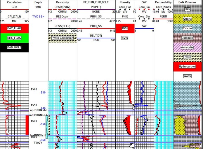
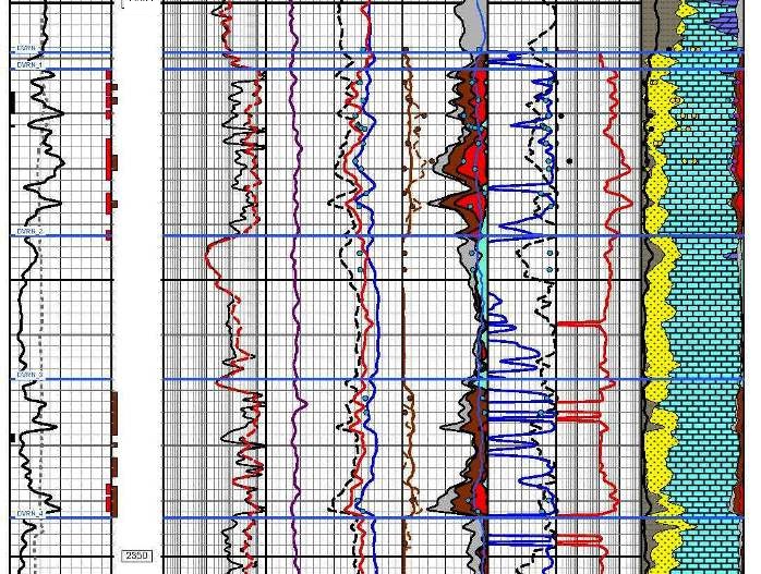
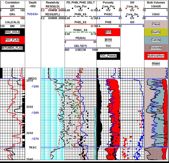
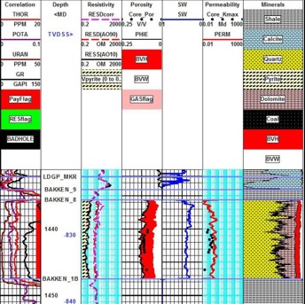
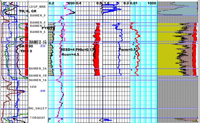
Bakken “Tight Oil” example has no kerogen in the productive sand /
silt section but very high kerogen content in the shales above and
below. Zone is radioactive due to uranium carried from the source
rocks during oil migration. Log example showing core porosity (black dots), core oil saturation (red dots).
core water saturation (blue dots), and permeability (red dots). Note
excellent agreement between log analysis and core data. Separation between red dots and blue
water saturation curve indicates significant moveable oil, even
though water saturation is relatively high (see text below for
explanation). NOTE that the organic rich Upper and Lower Bakken
Shales are much more resistive than the Middle Bakken Sand/Silt pay
zone due to the high TOC content in the shale. There is no
significant kerogen in the sand itself.
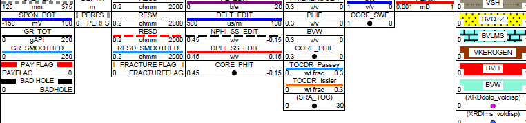
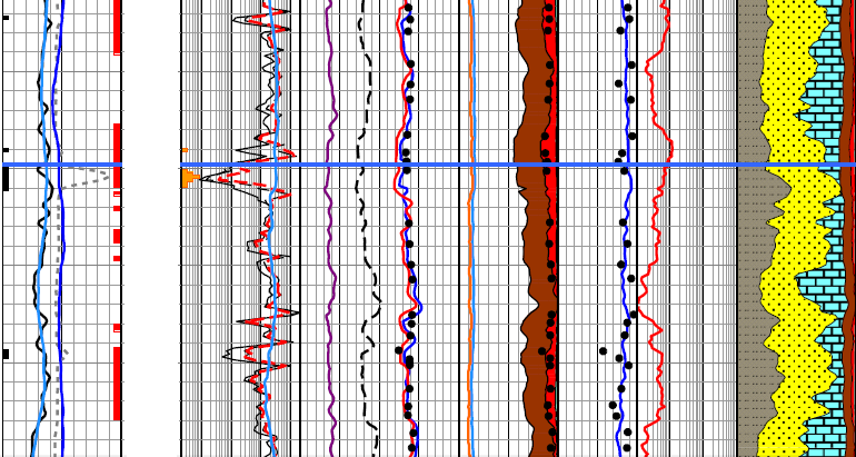
This is a genuine mature kerogen "shale oil" play from South America with lots of kerogen throughout
the reservoir, compared to the Bakken example that has virtually
none. The brown shading is the kerogen volume in the center track,
oil is red, water is light blue. Left edge of the red shading is
effective porosity from shale and kerogen corrected density neutron
porosity model. The core porosity and water saturation match the log
analysis values closely. TOC and clay volume from an offset well
were used to calibrate TOC models: Issler (orange) and Passey (blue)
on the left edge of the porosity track.
This Duvernay example shows the TOC from ECS and Issler methods
(left side of porosity track) and clay volume from ECS and total
gamma ray (left side of lithology track). The dark shading in the
porosity track is kerogen volume, red is oil, and light blue is
water. Water saturations are very low and agree with core data, as
does the porosity. CMR porosity is also available (blue curve in
porosity track). Pay flags for porosity > 3% (red bar) and for TOC >
2% (brown bar) are on left side of depth track. In this example, the
better porosity is not at the same depths as the high TOC content.
Where would you put the horixontal well?
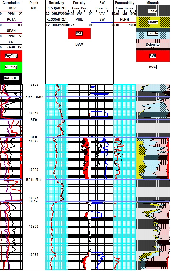
Example of a well in the Nordegg “tight oil” play. This well
is “tight” because of pyrobitumen filling most of the porosity. Core porosity (black dots) is
equivalent to effective porosity. Core oil saturation is very
high (red dots in saturation track, indicating a high fraction of
residual oil, except in the bottom 2 meters where some oil may be
moveable. Core water saturation is very
low (blue dots) as is computed water saturation. The red shading between the core porosity dots and the
water (white) may indicate moveable oil, but it could be a residual
liquid phase. “Pay Flag” is black
to indicate pyrobitumen, instead of red that would indicate mobile
fluids..
BAKKEN GEOLOGY
Oil in the Bakken in
southeastern Saskatchewan has migrated from mature Bakken source
rocks in North Dakota and Montana. The best reservoir is associated
with the Upper Middle Bakken Sandstone Facies (BF4). Average
porosity ranges from 14% to 16% and permeabilities are 20 to 80
millidarcies. The unconventional siltstone reservoir (BF2) averages
9% to 12% porosity and 0.01 to 1.0 millidarcies. In the deeper North
Dakota wells, porosity is somewhat lower but permeability may be
higher. All facies types have been exploited in different parts of
the Basin.
These facies were deposited during the late Devonian
and early Mississippian in what was then a tropical setting. The
sediment is believed to have an aeolian source and was blown into
the marine environment from the adjacent arid landmass to the east
and reworked into the various marine facies. The organic rich Upper
and Lower Bakken shales are the source rocks for the sand and silt
reservoirs.
The sands and silts are highly
dolomitic, averaging about 50% dolomite. In deeper wells, calcite
may replace some of the dolomite or infill some porosity.
Many of the dominant
features of the Bakken are below the resolution of logging tools and
are best seen in core photos and core logs, as shown below.
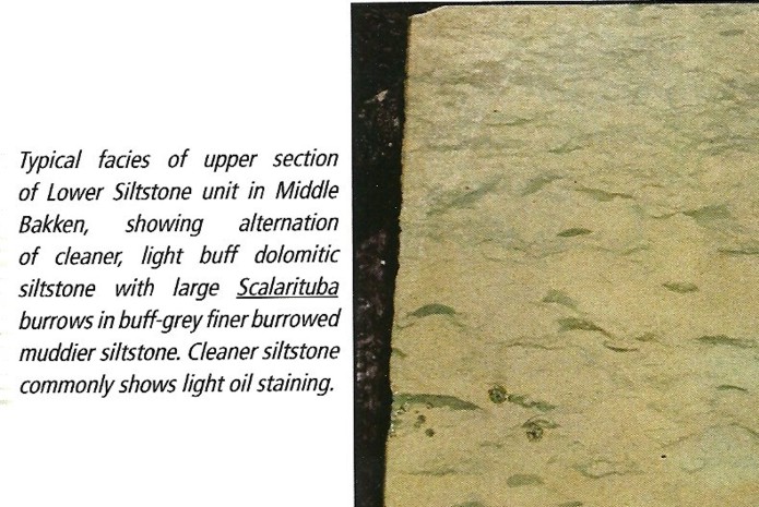
Core photo of Middle Bakken burrowed siltstone
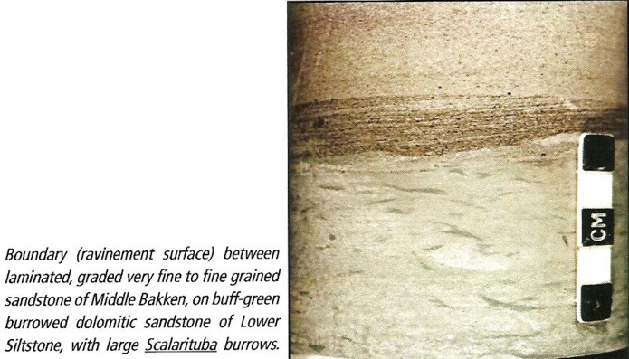
Core photo of Middle Bakken laminated fine grained sandstone
While
laminated shaly sands are best known, laminated porosity is also a
problem for log analysts. The Bakken and Montney reservoirs in
Canada are good examples. The illustrations below give a clear
example of how porosity logs and analysis results smooth out the
porosity variations, which in turn smooth out the saturation and
permeability answers. The latter is especially critical, since
productivity estimates for laminated reservoirs can be seriously
under-estimated because the high permeability streaks tend to be
ignored.
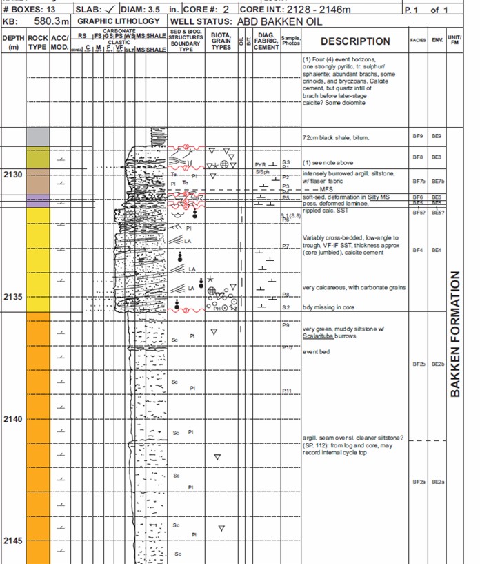
Core description log in a laminated Bakken sand. Upper half of
interval is highly laminated, lower half has thicker beds. See plot
of core data below. (Illustration courtesy Graham Davies Geological
Consulting)
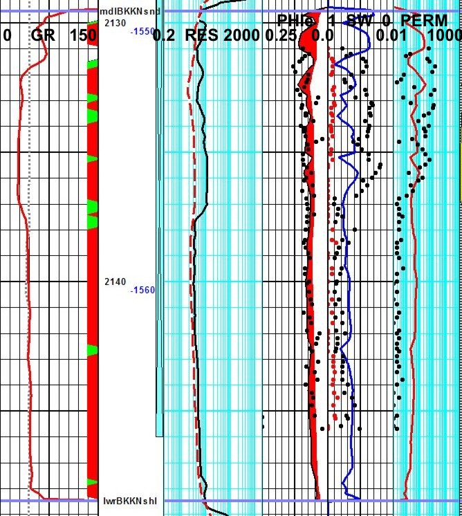
Expanded vertical scale log (grid lines = 1 meter) illutrating
different resolution of logs and core data.
Closely spaced core samples demonstrate laminated nature of Bakken
sand, compared to the running average created by well logs. Distinct
coarsening upward and fining upward sequences can be seen in the
upper half of core (grid lines are 1 meter). The lower half of the
cored interval is less laminated, so porosity and permeability
variations are smaller. Longer running average on resistivity log
makes water saturation even more difficult to assess and comparison
to core is worse than for porosity and permeability
Logs and core are for same well as core description shown above.
In
Saskatchewan, the naturally low resistivity in Bakken pay zones is
further aggravated by thin clay laminations, clay filled burrows,
laminated porosity, and dispersed pyrite.
Even more
confusing is the water resistivity variation on the northwest and
northeast edges of the Basin. Here, wet wells have higher
resistivity than oil wells further south because the water
resistivity is 5 to 20 times higher than deeper in the Basin. This
results from fresher water recharge from the Black Hills of North
Dakota. An adequate production testing program is the only solution
to this issue, as there is no log analysis model that will predict
water resistivity in this reservoir.
Water salinity in the deeper North Dakota wells reaches 325,000 ppm,
making for exceedingly low water resistivity. In Saskatchewan,
salinity is usually at 200,000 ppm or more, but can be as low as
25,000 in the recharge area. Pore geometry in the deeper parts is
more intergranular in texture and irreducible water saturation is
lower than in Saskatchewan.
Typical SW in
Saskatchewan averages 50% grading southward to about 30% in the
deeper North Dakota wells. Very low apparent SW in Saskatchewan
usually means fresh water recharge, possibly with some residual oil.
The "best-looking" wells are actually water producers, but have
measured resistivity values 2 to 4 times higher than productive oil
wells. Water resistivity values are sparse, so any water recovery
should be sent to the lab and analyzed.
The low
resistivity, high radioactivity, large density neutron separation
caused by dolomite and pyrite, and the high PE value (near 3)
conspire to make the zone look like shale on logs. Worse, some
literature continues to name the producing zone the Bakken Shale,
even though we know the Middle Bakken is a radioactive dolomitic
sand or siltstone. These conflicts in the conventional data suggest
strongly that some special core analysis should be done, namely
electrical properties, capillary pressure, X-Ray diffraction and
thin section mineralogy, and anything else that can help explain the
petrophysical response to these complex rocks.
The Bakken is
now the biggest oil play in North America, and may ultimately be the
largest ever found, even larger than Alaska North Slope. It is
sometimes termed an "unconventional" reservoir, due to the low
permeability of the siltstone intervals. In North Dakota, it is also
called a "resource" play because the oil was formed in place (from
the Upper and Lower Bakken Shales), although in Saskatchewan the oil
migrated from the deeper parts of the basin, and is not strictly
speaking a resource play there. Alberta and Montana is also probably
a resource play, but few facts have been published so it is hard to
tell.
Vertical
wells are not overly prolific due to the low intrinsic permeability
of the silty sand, but most horizontal wells do OK. In the deep,
hot, over-pressured region in North Dakota, some wells are flowing
1000 to 2000 barrels per day.
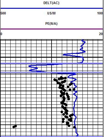 Core
analysis techniques, in particular the sampling interval, are
important in assessing tight oil or gas. Many, like the Bakken and
Montney plays, show a laminated porosity sequence. It is easy to
pick only the best sands, or otherwise obtain unrepresentative
samples. Since permeability is an exponential function of porosity
(as a general rule), small porosity variations make a big
difference in productivity estimates. The detail matters, and since
logs average about 1 meter of rock, log analysis permeability is
often pessimistic, even though the average porosity is correct. At
the right is the core and sonic log data for a Bakken well, showing
that the log cannot track the fine detail seen in the core. Many
core analyses take far fewer samples, so the laminated nature of the
reservoir is masked by too coarse a sample interval. Core
analysis techniques, in particular the sampling interval, are
important in assessing tight oil or gas. Many, like the Bakken and
Montney plays, show a laminated porosity sequence. It is easy to
pick only the best sands, or otherwise obtain unrepresentative
samples. Since permeability is an exponential function of porosity
(as a general rule), small porosity variations make a big
difference in productivity estimates. The detail matters, and since
logs average about 1 meter of rock, log analysis permeability is
often pessimistic, even though the average porosity is correct. At
the right is the core and sonic log data for a Bakken well, showing
that the log cannot track the fine detail seen in the core. Many
core analyses take far fewer samples, so the laminated nature of the
reservoir is masked by too coarse a sample interval.
 TIGHT OIL SHALE VOLUME CALCULATIONS
The Bakken is radioactive due mainly to uranium that migrated with
the oil. This can be identified with a spectral gamma ray log and it
should always be run when penetrating radioactive sands. Sadly, it
is often not requested, even though the service is cheap and costs
no extra rig time.
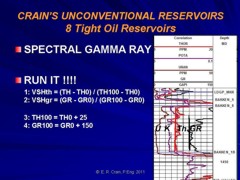
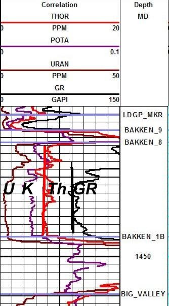
Spectral gamma ray log shows
Uranium (U), Potassium (K), Thorium (Th), and standard gamma ray (GR).
Red vertical line is TH0, the clean line for the Thorium curve, and
the black vertical line is GR0, the clean line for the GR curve.
Bakken 8 is top of sand and Bakken 1B is base of sand. 
The Thorium curve is best for shale volume calculations. The SP is
flat and useless, Density neutron separation is mostly due to
dolomite so it cannot be used. The gamma ray can be used in the
absence of the Thorium curve by assuming Uranium content is
constant.
1: VSHth = (TH - TH0) / (TH100 - TH0)
2: VSHgr = (GR - GR0) / (GR100 - GR0)
The Clavier correction to the gamma ray result is often used to
smooth out minor variations in uranium content that make the gamma
ray look "noisy":
3: VSHclavier = 1.7 - (3.38 - (VSHgr + 0.7) ^ 2) ^ 0.5
Choose VSHth in preference to VSHgr or VSHclavier when the thorium
curve is available. This becomes Vsh for all future calculations.
The clean lines TH0 and GR0 are
easy to pick (red and black lines on the illustration). Shale lines
are harder as they are often off-scale to the right or buried under
a plethora of backup curves. In the absence of a good pick from the
log, use:
4: TH100 = TH0 + 25
5: GR100 = GR0 + 150
Adjust the constants to suit your
local knowledge.
IMPORTANT: Remember that all log analysis models for TOC are
calibrated to standard geochemistry lab data that often do not
discriminate between kerogen and pyrobitumen. Either or both may be
present. Both have variable but fortunately similar physical
propertiees so converting log derived TOC to "kerogen" may actually
be a conversion to pyrobitumen or a mixture of the two components.
In the following material, you may want to substitute the words
"Organic Matter" for "Kerogen" to be more general.
KEROGEN volume
Some tight oil / shale oil plays contain kerogen,
just like shale gas plays. Little of the adsorbed gas in the kerogen
will move so we do not calculate adsorbed gas. But the kerogen does
affect our porosity calculation i so we must calculate and account
for the kerogen.
Kerogen volume is calculated by
converting the TOC weight fraction derived from density vs
resistivity or sonic vs resistivity methods, calibrated to
geochemical lab data.
0: Wtoc = TOC% / 100
5: Wker = Wtoc / KTOC
6: VOLker = Wker / DENSker
7: VOLma = (1 - Wker) / DENSma
8: VOLrock = VOLker + VOLma
9: Vker = VOLker / VOLrock
Where:
KTOC = kerogen correction factor - Range = 0.68 to 0.90, default
0.80
Wker = mass fraction of kerogen (unitless)
DENSker = density of kerogen (kg/m3 or g/cc)
DENSma = density log reading (kg/m3 or g/cc)
VOLxx = component volumes (m3 or cc)
Vker = volume fraction of kerogen (unitless)
DENSker is in the range of 0.95 to 1.45 g/cc (975 to 1450
kg/m3), similar to good quality coal.
Default = 1.26 g/cc (1200 kg/m3)
TIGHT OIL POROSITY CALCULATIONS
Even though the Bakken is a complex mixture of quartz, dolomite,
calcite, and sometimes pyrite, with a little clay, the standard
density neutron complex lithology crossplot model works well:
6: PHIdc = PHID
– (Vsh * PHIDSH) – (Vker * PHIDker)
7: PHInc = PHIN
– (Vsh * PHINSH) – (Vker * PHINker)
8: PHIe
= (PHInc + PHIdc) / 2
TIGHT OIL WATER SATURATION CALCULATIONS
Since there is little clay, the Archie model can be used, although
it costs nothing extra to use a shale corrected saturation equation
such as Simandoux or Dual Water:
9:
IF PHIe > 0.0
10: THEN C = (1 - Vsh) * A * (RW@FT) / (PHIe ^ M)
11: D = C * Vsh / (2 * RSH)
12: E = C / RESD
13: Sws = ((D ^ 2 + E) ^ 0.5 - D) ^ (2 / N)
14: OTHERWISE Sws = 1.0
Electrical properties variations
between facies and with depth or diagenesis are not published. This
lab work is worth the effort, as considerable increases in oil in
place are possible with small reductions in M and N values.
Tight oil and shale oil reservoirs are not "average" sandstones, so the electrical properties must be varied from
world average values in common use (A = 1, M = N = 2.0). To get
log analysis Sw to match lab data, much lower values are needed. Typically, A =
1.0 with M = N = 1.5 to 1.8. Unless lab derived properties are
available, vary M and N to obtain a good match to core Sw. If core
Sw is not available, the recommended default is M = N = 1.7.
Fresh
water recharge in the north can confuse log analysis results, so a
production test is essential before drilling any horizontal wells.
TIGHT OIL PERMEABILITY CALCULATIONS
There is no strong correlation between porosity and permeability has
been seen. The illustrations below show the scatter is large. The
Wyllie Rose equation gives rational values and can be tuned to fit
smoothed core data:
15: Kmax = 100 000 * (PHIe^6) / (SWir^2)
Permeability versus porosity scatter
plots for North Dakota well (left) and Saskatchewan well (right).
The scatter suggests microfractures.
TIGHT OIL Lithology CALCULATIONS
 How
do we know which minerals to use in the petrophysical log analysis?
Detailed sample descriptions are a good start. Both X-Ray diffraction data and thin section point counts can be
used. Both methods are considered semi-quantitative and come from
tiny samples compared to the volume measured by logs. So we don't
get too excited about obtaining a close numerical match . How
do we know which minerals to use in the petrophysical log analysis?
Detailed sample descriptions are a good start. Both X-Ray diffraction data and thin section point counts can be
used. Both methods are considered semi-quantitative and come from
tiny samples compared to the volume measured by logs. So we don't
get too excited about obtaining a close numerical match .
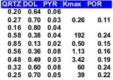
Mineral and core
analysis summary for a Bakken reservoir
Standard 3-mineral models using PE, density, and neutron data are
used with appropriate parameters for the selected minerals.
Multi-mineral solvers can be used if spectral gamma ray data is
available. In this case, shale volume would be derived also.
PYRITE CORRECTIONS
Pyrite is a
conductive metallic mineral that may occur in many different
sedimentary rocks. It can reduce measured resistivity, thus
increasing apparent water saturation. The conductive metallic
current path is in parallel with the ionic water conductive
path. As a result, a correction to the measured resistivity can
be made by solving the parallel resistivity circuit.
Although the math is simple, the parameters needed are not well
known. The two critical elements are the volume of pyrite and the
effective resistivity of pyrite. Pyrite volume can be found from a
two or three mineral model,
calibrated by thin section point counts or X-ray diffraction data.
The
resistivity of pyrite varies with the frequency of the logging tool
measurement system. Laterologs measure resistivity at less than 100
Hz, induction logs at 20 KHz, and LWD tools at 2 MHz. Higher
frequency tools record lower resistivity than low frequency tools
for the same concentration of pyrite. The variation in resistivity
is caused by the fact that pyrite is a semiconductor, not a metallic
conductor. It is nature's original transistor, and formed the main
sensing component in early radios.
Typical resistivity of pyrite
is in the range of 0.1 to 1.0 ohm-m; 0.5 ohm-m seems to work
reasonably well. The effect of pyrite is most noticeable when RW is
moderately high and less noticeable when RW is very low.
The
math is easiest when conductivity is used instead of resistivity:
16: CONDpyr = 1000 / RESpyr
17: CONDcorr = 1000 / RESD - CONDpyr * Vpyr
18: RESDcorr = 1000 / CONDcorr
The corrected resistivity can be plotted versus depth, along
with the original log.
Corrected water saturation will always be lower or equal to the
original Sw.
If CONDcorr goes negative, lower Vpyr or raise RESpyr
RESERVOIR QUALITY FROM CAP PRESSURE
A
capillary pressure (Pc) data set, along with some
calculated parameters, is summarized in the table
below.
|
CAPILLARY PRESSURE SUMMARY |
|
Sample |
Depth |
Perm |
PHIe |
SWir |
SWir |
PHI*SW |
PHI*SW |
sqrt/PHIe) |
Pore Throat |
|
|
m |
mD |
|
425m |
100m |
425m |
100m |
|
Radius um |
|
Bakken |
|
|
|
|
|
|
|
|
|
|
1 |
03.5 |
2.40 |
0.118 |
0.12 |
0.19 |
0.014 |
0.022 |
4.51 |
1.358 |
|
2 |
04.3 |
0.24 |
0.137 |
0.62 |
0.94 |
0.085 |
0.129 |
1.32 |
0.036 |
|
3 |
04.5 |
0.32 |
0.139 |
0.39 |
0.64 |
0.054 |
0.089 |
1.52 |
0.100 |
|
4 |
05.2 |
0.77 |
0.149 |
0.31 |
0.62 |
0.046 |
0.092 |
2.27 |
0.113 |
|
Average |
04.4 |
0.93 |
0.136 |
0.36 |
0.60 |
0.050 |
0.083 |
2.41 |
0.402 |
|
|
|
|
|
|
|
|
|
|
|
|
Torquay |
|
|
|
|
|
|
|
|
|
|
5 |
16.8 |
0.05 |
0.163 |
1.00 |
1.00 |
0.163 |
0.163 |
0.55 |
0.008 |
|
6 |
20.4 |
0.07 |
0.145 |
0.59 |
0.97 |
0.086 |
0.141 |
0.69 |
0.038 |
|
7 |
21.8 |
0.09 |
0.174 |
0.79 |
0.96 |
0.137 |
0.167 |
0.72 |
0.019 |
|
8 |
23.8 |
0.03 |
0.157 |
1.00 |
1.00 |
0.157 |
0.157 |
0.44 |
0.009 |
|
9 |
31.4 |
0.07 |
0.138 |
0.83 |
0.98 |
0.115 |
0.135 |
0.71 |
0.017 |
|
Average |
24.4 |
0.07 |
0.154 |
0.80 |
0.98 |
0.124 |
0.150 |
0.64 |
0.021 |
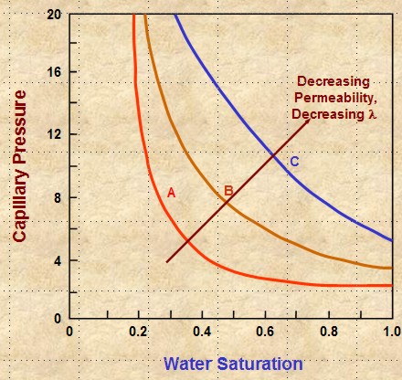 In
higher permeability rock, the cap pressure curve quickly reaches an
asymptote and the minimum saturation usually represents the actual
water saturation in an undepleted hydrocarbon reservoir above the
transition zone. In tight rock, the asymptote is seldom reached, so
we pick saturation values from the cap pressure curves at two
heights (or equivalent) Pc values) to represent two extremes of
reservoir condition. In
higher permeability rock, the cap pressure curve quickly reaches an
asymptote and the minimum saturation usually represents the actual
water saturation in an undepleted hydrocarbon reservoir above the
transition zone. In tight rock, the asymptote is seldom reached, so
we pick saturation values from the cap pressure curves at two
heights (or equivalent) Pc values) to represent two extremes of
reservoir condition.
Only sample 1 in the above table behaves close to
asymptotically, as in curve A in the schematic illustration at the
right. All other samples behave like curves B and C (or worse). The
real cap pressure curves for samples 1 and 2 are shown below.
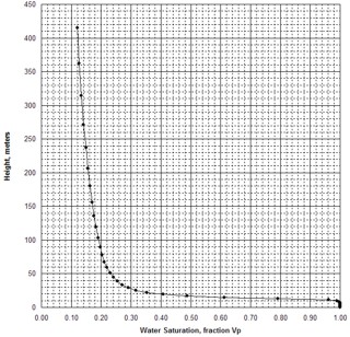
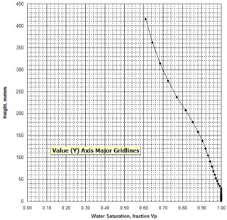
Examples of capillary pressure curves in good quality rock (sample 1
– left) and poorer quality rock
(sample 2 – right)
The summary table shows wetting phase saturation
selected by observation of the cap pressure graphs at two
different heights above free water, namely 100 meters and 425 meters
in this example. In this case, the 100 meter data gives water
saturations that we commonly see in petrophysical analysis of well
logs in hydrocarbon bearing Bakken reservoirs in Saskatchewan. This
is a pragmatic way to indicate the water saturation to be expected
when a Bakken reservoir is at or near irreducible water saturation.
The data for the 450 meter case is considerably lower and probably
does not represent reservoir conditions in this region of the
Williston Basin.
Two other columns in the table are
calculated from the primary measurements.
The first is the product of porosity times
saturation, PHI*SW, often called Buckle’s Number. It is considered
to be a measure of pore geometry or grain size. Higher values are
finer grained rocks. These values vary considerably in the Bakken,
between low and medium values, indicating the laminated nature of
the silt / sand reservoir. The values in the Torquay are uniformly
high, indicating that the reservoir is poor quality in all samples.
The second is the square root of permeability divided
by porosity, sqrt(Kmax/PHIe), which is another measure of reservoir
quality, directly proportional to pore throat radius and Pc. High
numbers represent good connectivity and low values show poor
connectivity. Again, the Bakken shows the variations due to
laminations, and the Torquay shows low values and unattractive
reservoir quality.
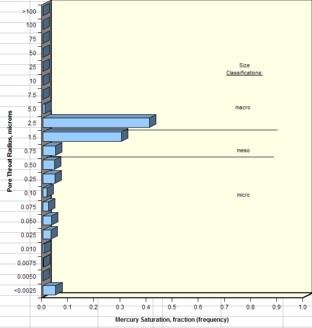
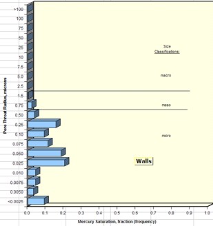
Examples of pore throat radius distribution
in good quality rock (sample 1 – left) and poorer quality rock
(sample 2 – right)
By comparing cap pressure and pore throat
distribution graphs from each sample with the quality indicator
values in the summary table, it becomes more evident as to which
parameters in a petrophysical analysis might be the best indicator
of reservoir quality. Since both Buckle’s Number and the Kmax/PHIe
parameter can be determined from logs, it has been relatively common
to assess reservoir quality from these parameters as a proxy for
capillary pressure and pore throat measurements.
However, in thinly laminated reservoirs like the
Bakken, this is not always possible since the logging tools average
1 meter of rock. This means we cannot see the internal variations of
rock quality evident in the core data.
BAKKEN EXAMPLES
Example 1: Bakken, SE Saskatchewan
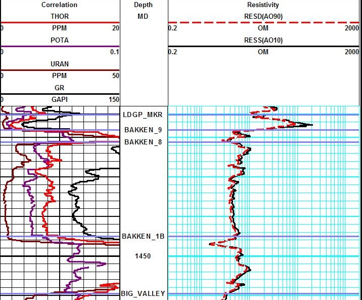
Resistivity log on low
resistivity, radioactive Bakken sand (4 ohm-m in best sand). Note high resistivity upper
and lower shales, which are the source rock for the oil in the sand.
These are "real" shales with gamma ray readings between 250 and
500
API units. Spectral GR shows low but significant uranium content in
sand and very high uranium
in the shales, associated with the kerogen content. The thorium
curve is the best clay indicator.
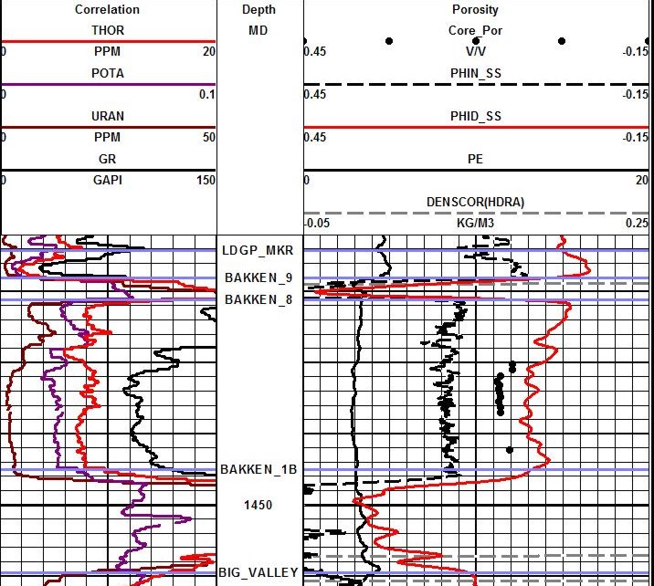
Density neutron logs on low
resistivity, radioactive, dolomitic Bakken sand. Note high apparent
porosity (almost coal values) in upper and lower shales. Density neutron separation and PE show a 50-50 mix of
quartz and dolomite with a few percent pyrite. XRD and sample
descriptions confirm this
analysis.
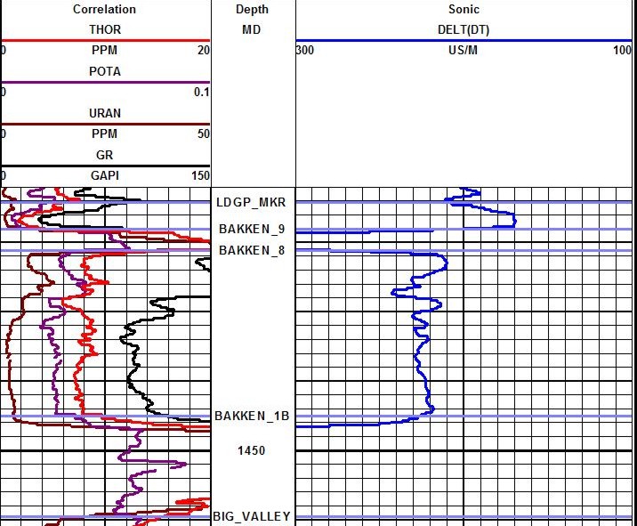
The
sonic log is also
useful in a 3 or 4 mineral model and for calculating porosity in
older wells that have no density neutron logs. Matrix travel time
needs to be calibrated to allow a match to core.
The answer plot illustrates the mineral mix and the good match to core
porosity and permeability that was achieved. The curves in the
correlation track are, from left to right, uranium, potassium,
thorium, total gamma ray.
Example 2: Bakken, SE Saskatchewan With Pyrite Correction
Here is a different well with the pyrite correction applied to the
resistivity log. The before and after
versions of the resistivity are shown in Track 2, along with the
pyrite fraction determined from a
3-mineral model using PE-density-neutron logs. The correction raises
the resistivity about 0.5
ohm-m and reduces water saturation by about 10%. Making the pyrite
more conductive would
raise RESD further, but as yet no one has provided any public
capillary pressure data in this area
to calibrate SW. The SWir from an NMR log would also help calibrate
this problem.
Example 3: Bakken, North Dakota
This example is from the deeper, hotter, overpressured part of the
Williston Basin. Depths are in feet, porosity and permeability are
lower than the Saskatchewan examples shown earlier, but the zone is
thicker. Water resistivity is very low due to saturated salt water
(320,000 ppm) and high temperature (200+F). Note the possibility of
hydrocarbons below the Lower Bakken Shale.
CARDIUM, VIKING, DUNVEGAN EXAMPLES
Example 4: Cardium, Alberta
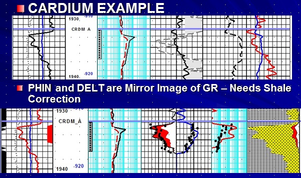
Many “Tight Oil” plays are really “Old Oil” plays, usually gas
expansion drive reservoirs with low recovery factors. Laminations
(seen here on the core porosity) and high shale volume suggest that
some of the perforated interval has not yet been produced. Whether
these wells produce gas only or gas plus oil depends entirely on
intrinsic permeability and oil gravity - low perm can only make gas,
higher perm can let out some oil. Stimulation may increase oil rate..
Example 5: Viking, Alberta
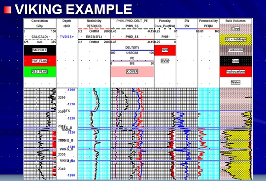
The Viking is also a laminated, shaly, gas expansion drive
reservoir with a low recovery factor on initial completion.
Horizontal wells with a modern stimulation (massive hydraulic frac
job) improve recovery factor and flow rates. Conventional
petrophysical models work well. Tight streaks act as baffles, not
barriers, and can only be seen in micrologs, resistivity image logs,
or detailed core descriptions.
Example 6: Dunvegan, Alberta
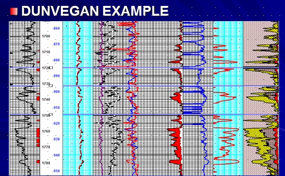
Another tight oil example is the Dunvegan, a multi-layer sequence of
fining upward and coarsening upward sequences with highly variable
shale volume and porosity. Tight laminations, seen on micrologs, but
not conventional open hole logs, reduce net pay.
|